Predicting the 2022 football world cup with R and Stan

⚽ ⚽ ⚽ ⚽ ⚽ ⚽ ⚽ ⚽ ⚽ ⚽ ⚽ ⚽ ⚽ ⚽ ⚽ ⚽

Author

Maurits Evers

Published

November 16, 2022

Introduction

A Stan-based Bayesian model is used to predict outcomes of the 2022 FIFA football world cup in Qatar. The model itself is fairly simple, and was adopted from the model introduced by Andrew Gelman on his blog “Statistical Modeling, Causal Inference, and Social Science” here and here. Andrew’s model was also used by Mitzi Morris in the “Bayesian workflows with CmdStanPy” workshop to predict results of the 2019 FIFA women’s world cup in France.

Warning

This is a work in progress. There may be bugs. There may be poor modelling & data choices. There may be both. As with all models & modelling approaches, there are inherent limitations of the model.

Interpret with caution!

Prerequisities

Load necessary R libraries, set Stan options and load R convenience functions.

Show the code

library(rstan)
library(tidyverse)
library(lubridate)
library(tidybayes)
options(mc.cores = parallel::detectCores())
rstan_options(auto_write = TRUE)
source("R/utils.R")

The model

In a nutshell, the model estimates score differentials and uses those to determine

the ranking of teams during the group stage, and
winners and losers during the quarter-finals, semi-finals and final.

The model has some similarities with the Bradley-Terry model, and infers team abilities from historical match data by considering prior team abilities (more precisely: the model estimates team abilities by partially pooling ability estimates toward a prior estimate). Prior team abilities are given by (standardised) ELO ratings. Team abilities are estimated based on the observed goal difference.

The model uses draws from the posterior distribution of team abilities to simulate the outcome of all matches, from the group phase all the way to the final. Predicted outcomes of the group phase matches are used to determine the winners and runner ups in every group that advance to the round of 16, and from there to the quarter finals, semi finals and finals. Therefore, the number of draws mimics the total number of simulated world cup tournaments played. With every draw, a set up teams can be identified at any stage of the world cup tournament all the way to the final winner.

Note

When simulating (predicting) tournament results, some key assumptions are made. For example, following the group phase matches, teams are ranked based on the sum of their score differentials across all games played. This is obviously not how winners and runner ups are determined according to FIFA World Cup 2022 regulations. However this method is straightforward to implement and offers a simple way to rank teams within every group.

Data

Team data

A CSV file with all 32 2022 WC football teams, their group associations and positions within their group is stored in ./data-raw/teams_by_group.csv.

ELO ratings were extracted from https://www.eloratings.net on 15 November 2022 and stored in a CSV file ./data-raw/elo_ratings_Nov22.csv in the code repository.

Team data with group information and ELO ratings are combined to give a countries dataset

Show the code

countries <- read_csv("data-raw/teams_by_group.csv") %>%
    left_join(
        read_csv("data-raw/elo_ratings_Nov22.csv") %>% select(team, rating), 
        by = "team") %>%
    mutate(ranking = rank(-rating, ties.method = "first"))
countries

Match data

Historical football match data are conveniently downloaded from Kaggle here (note that this requires a Kaggle account which is free). The dataset includes international football results from 1872 to 2022, and is stored in a CSV file ./data-raw/results.csv in the code repository. Historical match data are filtered to include only games

from 2020 onwards,
with teams now playing in the 2022 football WC, and
that were “non-friendly” matches (i.e. they were part of a football association’s tournament).

Show the code

matches <- read_csv("data-raw/results.csv") %>%
    filter(
        year(date) >= 2020,
        home_team %in% countries$team,
        away_team %in% countries$team,
        tournament != "Friendly")
matches

Note

Yes, the match data filtering employed here is fairly arbitrary. For example, excluding friendly matches lowers the average score difference (or conversely: teams tend to score more goals in friendly matches, leading to more extreme score differences). This in turn has an effect on estimating team abilities, which would have been higher if high score difference matches had been included.

Fitting the model

The Stan model file can be found in ./models/wc_qatar_full.stan in the code repository.

Show the code

fit <- fit_model(countries, matches, iter = 250000)

As explained previously, the model estimates team abilities and then simulates playing 1 million world cup tournaments from the group phase to the final, based on the inferred distribution of every team’s abilities. Estimates of teams and winners at every stage are stored in the fit object.

Predictions

Results of group phase

Based on the model fit, the end of the group phase has teams with the following final score differential distribution (Bayesian inference gives the full posterior distribution). The solid dots show the median values, the thick and thin horizontal lines denote the 66% and 95% quantile intervals, respectively.

Show the code

fit %>%
    spread_draws(final_score_diff[group, team_pos]) %>%
    mutate(group = recode(
        group, 
        `1` = "A", `2` = "B", `3` = "C", `4` = "D", 
        `5` = "E", `6` = "F", `7` = "G", `8` = "H")) %>%
    left_join(countries, by = c("group", "team_pos")) %>%
    ggplot(aes(final_score_diff, y = fct_reorder(team, final_score_diff))) + 
    stat_pointinterval() + 
    facet_wrap(~ group, scales = "free_y") +
    theme_minimal() +
    labs(
        title = "Final score differential of teams per group at the end of the group phase",
        x = "Final score differential",
        y = "") +
    theme(plot.title.position = "plot")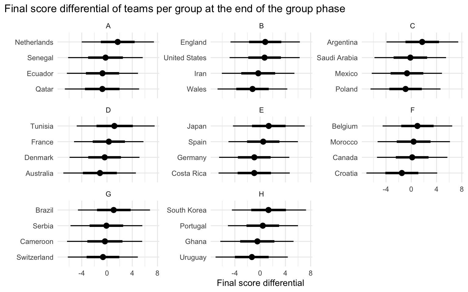

The two teams with the highest positive score differentials are named the winners and runner-ups of every group and advance to the quarter finals.

Semi-finals

The top 20 most probable semi-finals are shown in the following plot.

Show the code

fit %>%
    spread_draws(teams_sf[match, team_idx]) %>%
    left_join(
        countries %>% select(ranking, team), 
        by = c("teams_sf" = "ranking")) %>%
    select(-teams_sf) %>%
    pivot_wider(names_from = team_idx, values_from = team) %>%
    unite(match, `1`, `2`, sep = " : ") %>%
    group_by(match) %>%
    summarise(prob = n()) %>%
    ungroup() %>%
    mutate(prob = prob / sum(prob)) %>%
    arrange(desc(prob)) %>%
    head(n = 20) %>%
    ggplot(aes(prob, fct_reorder(match, prob))) + 
    geom_point() +
    geom_segment(aes(x = 0, xend = prob, yend = fct_reorder(match, prob))) +
    theme_minimal() + 
    scale_x_continuous(labels = scales::percent) +
    labs(
        title = "Top 10 most probable semi-finals",
        x = "Probability",
        y = "Teams") +    
    theme(plot.title.position = "plot")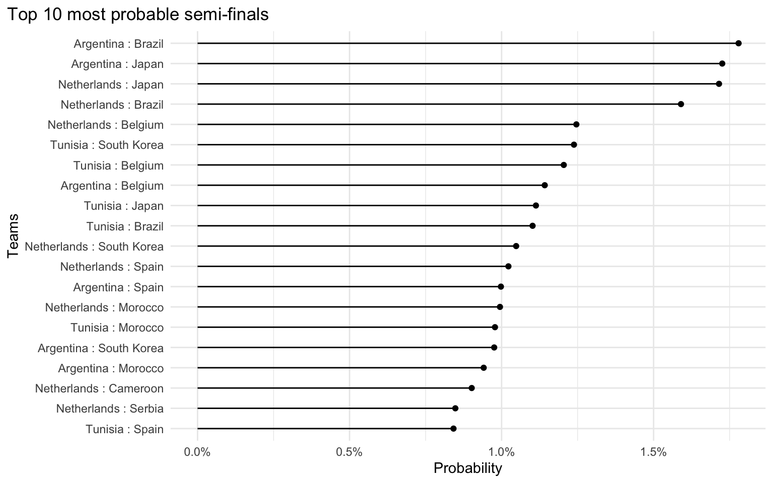

Note

Probabilities are very small because of the way that the model simulates WC tournaments, which leads to a large range of possible team combinations at the different stages of the tournament. So as far as the most probable semi-final matches are concerned, it’s better to look at relative differences between the match probabilities. For example, the semi-final Netherlands vs. Brazil is around 1.5 times as likely as the semi-final Netherlands vs. Spain.

Finals

Team probabilities for winning the 2022 football world cup are given below.

Show the code

fit %>%
    spread_draws(winner_ff) %>%
    left_join(countries, by = c("winner_ff" = "ranking")) %>%
    group_by(team) %>%
    summarise(prob = n()) %>%
    ungroup() %>%
    mutate(prob = prob / sum(prob)) %>%
    ggplot(aes(prob, fct_reorder(team, prob))) + 
    geom_point() +
    geom_segment(aes(x = 0, xend = prob, yend = fct_reorder(team, prob))) +
    theme_minimal() + 
    scale_x_continuous(labels = scales::percent) +
    labs(
        title = "Probability of winning the 2022 football WC",
        x = "Probability",
        y = "") +
    theme(plot.title.position = "plot")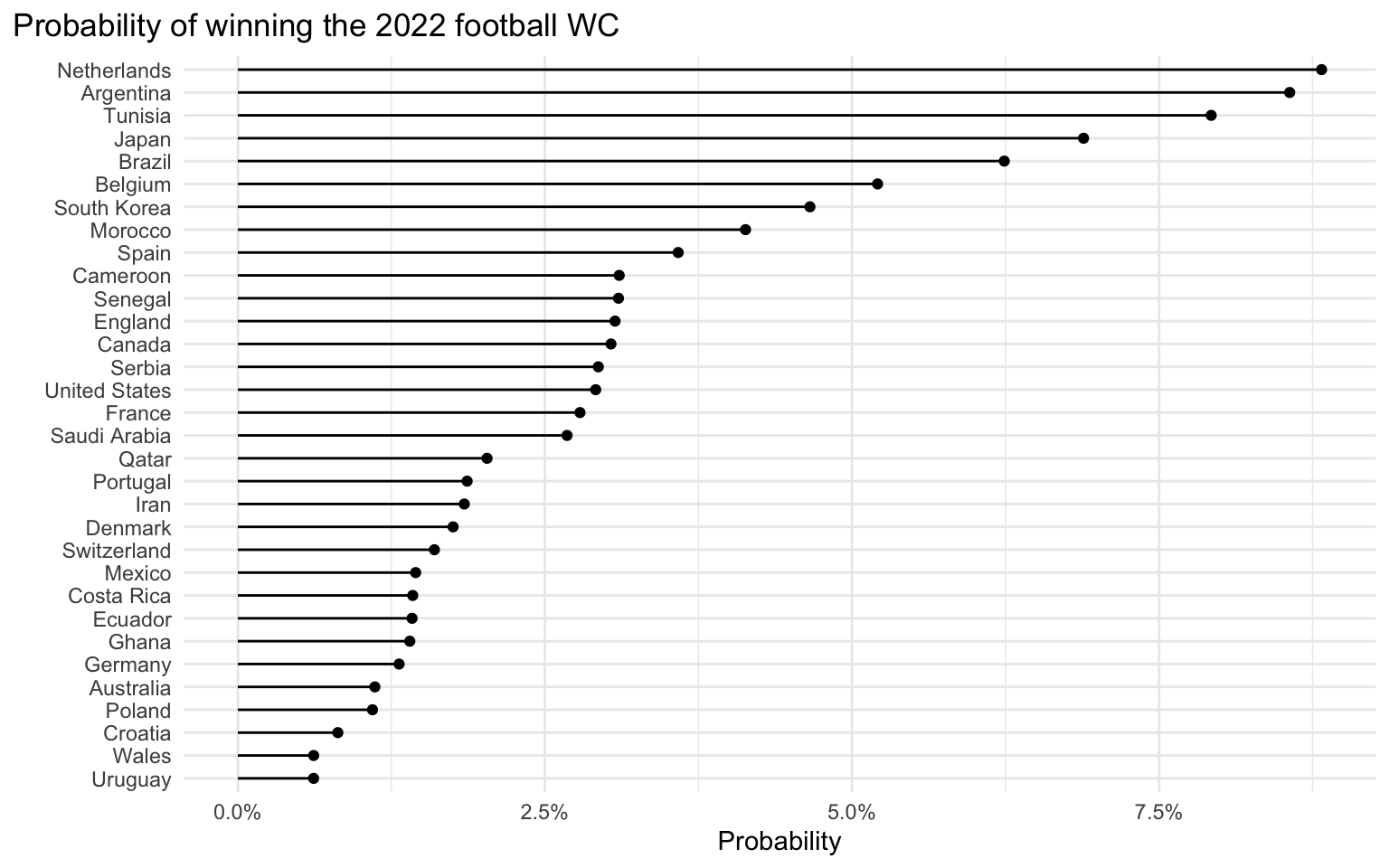

Note

Probabilities of individual teams winning the world cup are all fairly low. This is a combination of the way that historical match data were selected (for example, including friendly matches would have meant larger observed score differences which in turn would have resulted in more extreme team ability estimates), and the fact how the model simulates WC tournaments.